Lecture 2#
Ergodic hypothesis#
We discussed a MD simulation related to liquid Ar previously. In this simulations, we modeled Ar liquid at 95 K using ~900 atoms. If you consider a vessel full of liquid Ar with a volume of 10\(^{-3}\) \(m^3\), it will contain 1.4096 kg of Ar or 2.125*10\(^{25}\) Ar atoms. Considering that this is a fluid, the arrangement of atoms is not periodic either. These atoms could arrange themselves in so many ways. If we chose any ~900 atoms from this vessel, we would find a very large number of configurations or states. The macroscopic properties that we observe are a result of an average of these configurations. How does our system of ~900 atoms would predict the macroscopic properties?
Of course, we can model a large number of configurations and then take an average to calculate the property of interest. However, a better solution is given by the ergodic hypothesis. It states that over long periods of time, all the states of the system are equiprobable. In other words, time average of a property is same as sampling multiple states. As you can imagine, this is really useful!
Ensembles#
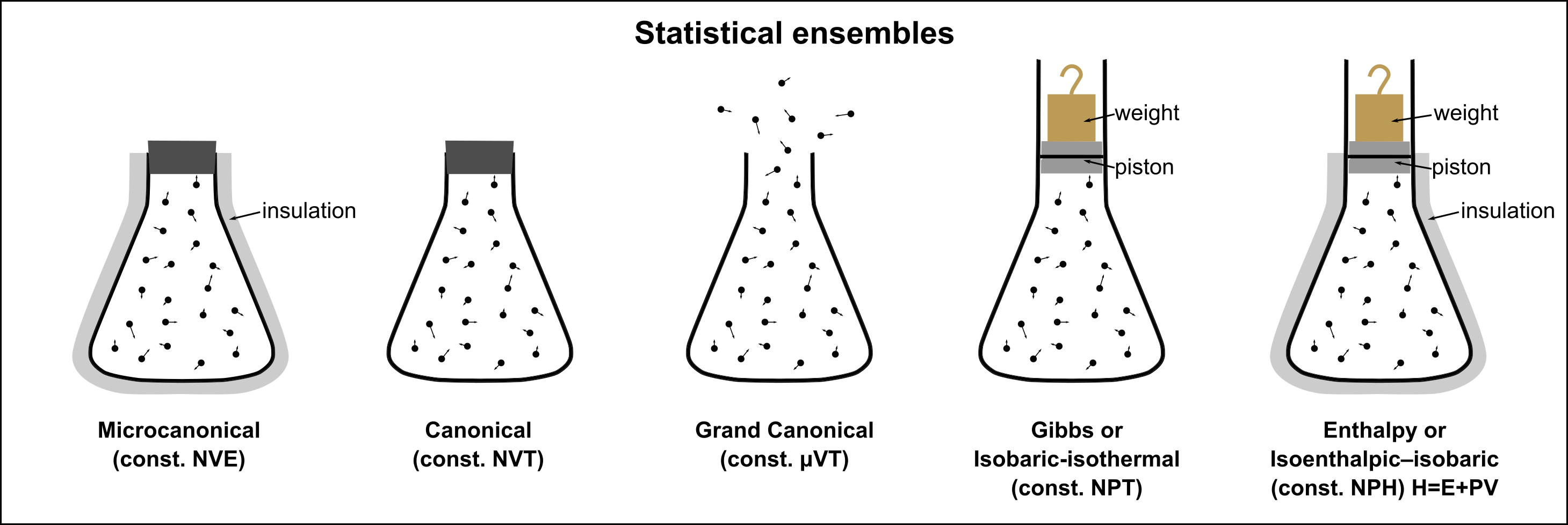
Our MD simulations code described earlier conserved the number of particles (N), volume (V) and total energy (E) of the system. This is referred to as the NVE or the microcanonical ensemble. It is often more convenient to perform simulations at constant temperature or pressure. This is achieved through NVT and NPT ensembles respectively. Let us consider the NVT ensemble.
As the name suggests, this ensemble is used to implement isothermal conditions. In this ensemble, the simulation system is kept in contact with a heat bath to maintain the temperature of the system. Note that the energy of the system is allowed to change. This effect is achieved using thermostats. Thermostats are the algorithms that part of every standard MD code used to maintain the temperature of the system. Anderson thermostat, Berendsen thermostat, Nose-Hoover thermostat, and Langevin (stochastic) thermostat are some of the popular examples.
If we want to maintain the temperature of the system, an easy way would be to reassign the velocities of the atoms as per the temperature. The kinetic energy and particle velocity distribution of a system can be determined using Boltzmann distribution for the given temperature. We can fix the velocities of the particles at every time step as per this distribution to keep the total kinetic energy constant. However, this is not our aim. We want the system to behave as if in contact with a large heat bath. The above method could result in biasing the particle dynamics which could lead to nonphysical results. We want the temperature of the system to be the desired temperature while allowing for local fluctuations.
Let us consider the example of the Berendsen thermostat. In this method, the velocities are scaled at each time step so that the rate of change of temperature is proportional to the difference between the system temperature and the target temperature.
Here, \(\tau\) is the coupling parameter. This parameter will decide how strongly the system temperature is controlled. You would not want to control it too strongly or too weakly. A typical rule of thumb is to make \(\tau\) 100x larger than your time step. However, this specification could change based on your simulation. If you want to be sure, you can always try different values for \(\tau\) or the coupling parameters and make sure that you are not observing nonphysical effects. Similar effect can be achieved for pressure by using a barostat.
The following figure shows a visual representation of different ensembles.

Fig. 3 Visual representation of different ensembles. (source: Wikipedia)#
Interatomic potentials#
We used the L-J potential to calculate density of an inert gas. It described the energy between a pair of particles as a function of interatomic distance. This description is well and good for monoatomic species or when representation of a species as hard sphere is sufficient. Realistically, a large number of problems involve complex molecules. These complex molecules need the description of bonds, angles and dihedrals. The complex shapes also mean that we need to consider rotational and vibrational motion along with translational motion. Also, physical systems involve more complex interactions. Strong interactions such as covalent, metallic and ionic bonding are necessary to capture the reactivity of the system. Additionally, we also need to consider weak interactions such as hydrogen bonds, permanent dipoles and vdWaals interactions. Including all these interactions naturally leads to a complex form of classical potential. Listed below are different bonded and non-bonded interactions typically considered in interatomic potentials
Bond stretch#
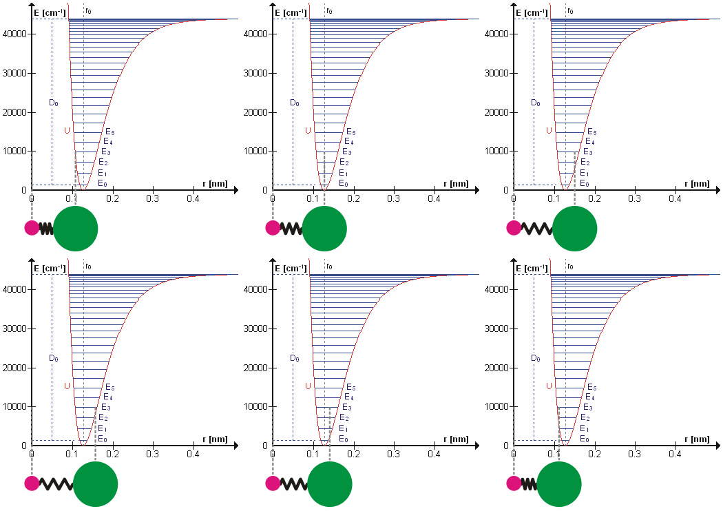
At finite temperatures, bonded atoms vibrate or chemical bond lengths deviate from their equilibrium values. These vibrations typically occur at certain frequencies characteristic to the different vibrational excitation levels for the bond. The vibrational excitations also increase the energy of the bond. After reaching sufficiently high energy (bond dissociation energy), the bond would eventually break. If interested in non-reactive application, the vibrational motion can be approximated sufficiently by harmonic approximation. For example, the energy of the HCl molecular bond can be reasonably approximated upto \(E_2\) or \(E_3\) by the following expression
As \(r_{HCl}\rightarrow\infty\),\(U(r_{HCl})\rightarrow\infty\). Hence, this expression will not be able to express the breaking of the bond though. A better approximation is represented by Morse potential defined below. A lot of the non-reactive force fields still use either harmonic approximation or it’s modified form by including quadratic term in the equation above. The reason for this is the higher computational cost of calculating exponential.

Fig. 4 Molecular vibration of HCl. (source: Wikipedia)#
Similar to bond stretch, we also need to consider angle, dihedrals as well as non-bonded interactions like
